Tutorials > Too many differences

This tutorial explains how to minimize the number of differences using the filter function.

When comparing cells Synkronizer first looks at the data type of the cells (Numbers/Text/Date/Boolean/Error etc) and only then compares the actual content. If the data type and the content are not completely equal a difference will be reported.

Sometimes this is too precise for your purpose and you get too many differences.. e.g. you don't care about differences like "Customer" and "CUSTOMER" or 123 and "123"

Then you can use Filters to instruct Synkronizer to be less precise. This page will show you how to do that.

1.	Download the example files from the webpage: http://www.synkronizer.com/files/examplefiles.zip

2.	Extract the zip file and copy the Excel files to a folder of your preference.

3.	Open Excel and start Synkronizer.

4.	Select the files Master.xls and Update.xls.

5.	Select the worksheets "TDM1" and "TDM2" and start then the comparison process.

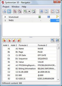
6.	The Navigator form is displayed which determined 500 differences:

7.	As you scan see from the first couple of differences the data in the first files is "Proper" in the other it is "UPPER".

8.	Let's set a filter to "Ignore the case". Open the menu Project » Settings.

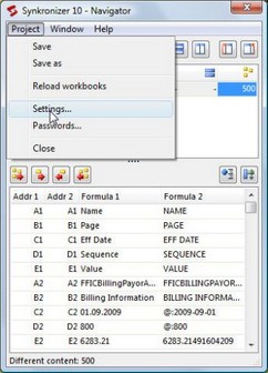
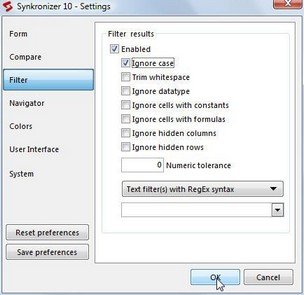
9.	On the form Select "Filters". First check "Enabled" then check the Option "Ignore Case" Close the form by clicking the Ok button.

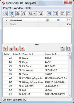
10.	You go back to the Navigator form. Click the Button "Run the comparison again" (2nd button in the top row, see cursor)

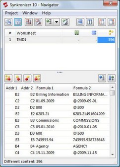
11.	We now have 396 differences left.

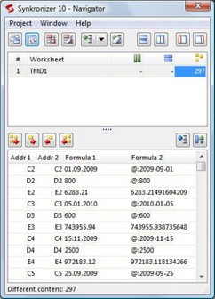
12.	Closer inspection will show that the differences in Column B are caused by trailing spaces in the "Update" file. Repeat the steps 7-10 and add a check next to the filter option "Trim Whitespace". You should now have 297 differences left.

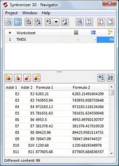
13.

Now look at the differences. You'll notice that some cells are displayed with the @-sign. This is an indicator for cell content that is stored as text but can be converted to a Number, a Date or a Boolean. These differences can be filtered by ignoring the data type.
Repeat the steps 7-10 and add a check next to the filter option "Ignore data type". You should now have 99 differences left.
[Remark: Ignore Datatype will only work if the text can be converted using the current system locale (regional settings)]

tutorial_c7_en

14.

We now have only differences in column E remaining. You'll quickly see that the numbers in Master are rounded, but the numbers in Update are not.(although in the worksheet the extra precision is not displayed due to a number format). These differences can be ignored by setting a numeric tolerance. Go to the Filters page on the Settings form and set a value of 0.01 in the box for "Numeric Tolerance".

tutorial_c8_en

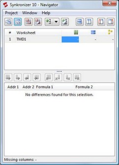15.	No more differences found!

Too many differences (using filters)